Model to Script to Tool: the "Holy Trinity"

I have been doing some work for a junior mining company recently involving creating Volume/Elevation curves (see my last post). This work is accomplished in ArcGIS using Spatial Analyst and 3D Analyst which works very well but requires many steps. Over the course of this project, however, I have built a number of Python scripts that are now embedded as tools in a new toolbox in ArcMap. So I am going to take this opportunity to briefly discuss how easy it really is to create sophisticated Python geo-processing scripts in Arc and give a little example of how I recommend approaching this task.

First of all I would just like to say that ArcGIS is still the most powerful GIS in my opinion (yes I am still a fan of open source but you can't argue with the benefits of having a large budget to develop good software). I like Arc not so much for it's ability to perform the geo-processing functions but more for the ancillary tools that help you find the appropriate tools and perform these tasks. Arc has built in search capabilities and very good documentation to allow users with a wide variety of skill levels find the appropriate tools. On top of that, there is a very well developed modeling and scripting environment that gives the user the capability to reproduce these tasks in a relatively easy manner.

Ok, now that's been said lets get on with the main purpose of this post, to show how easy it is to create a tool in ArcGIS using the modeling and scripting environments. For this example I thought I'd use the volume elevation curve tool created for the project I mentioned earlier. I will be making reference to a number of steps that may not be clear if you haven't performed this analysis before but you can read my previous post for clarification.

The Model

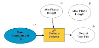
So over the years I have found that the easiest way to start any Python scripting in Arc is to look at the modeling environment first and see if the task can be done in there. You may ask "why worry about a Python script if you can create a model", but if you need to add some iterationFigure 1: Surface volume model

to the process (e.g. performing the analysis on successive elevations), for example, then you need to do this with a script. So I started by creating the model shown in Figure 1. The key here is to notice that I have created a number of "model parameters" which will show up as argument variables (sys.argv[]) when the model is exported to Python. These arguments will allow you to attach the fields from a custom tool to them giving the user the flexibility to add their own data, assign a range of elevations to the plane height variable and specify the output location for the delimited text file. You will also notice that there are two height variables (Min Plane Height and Max Plane Height) but only one is actually attached to the model. This is because we are planing to have an iterative model that starts at the bottom of the surface (e.g. 0 cu.m volume) and works it's way up to the top. This requires that we allow the user to assign a lower value and an upper value but because this model is only a single instance of the volume command, it can take only one value. Don't worry though, we will add the iterative properties when we edit the script. Once you have the model the way you like you can export it to a Python script (Model -> Export -> To Script -> Python). Before doing this though, I suggest testing the model to ensure it works to avoid spending an unreasonable amount of time on the scripting.

The Script
Now that we have a script you can open it up in IDLE or whichever Python editing environment you like. The script will look something like Figure 2 after it is first exported.

# ---------------------------------------------------------------------------
# sample_model_script.py
# Created on: Thu Sep 02 2010 04:23:36 PM
# (generated by ArcGIS/ModelBuilder)
# Usage: sample_model_script
# ---------------------------------------------------------------------------

# Import system modules
import sys, string, os, arcgisscripting

# Create the Geoprocessor object
gp = arcgisscripting.create()

# Check out any necessary licenses
gp.CheckOutExtension("3D")

# Load required toolboxes...
gp.AddToolbox("..Toolboxes/3D Analyst Tools.tbx")

# Script arguments...
Output_Text_File = sys.argv[1]

Dam_Containment_Tin = sys.argv[2]

if Dam_Containment_Tin == '#':
     Dam_Containment_Tin = "defa" # provide a default value if unspecified

Min_Plane = sys.argv[3]

Max_Plane_Height = sys.argv[4]

# Local variables...

# Process: Surface Volume...
gp.SurfaceVolume_3d(Dam_Containment_Tin, Output_Text_File, "BELOW", Min_Height, "1")

Let's run through the components of this script. First of all you have to import the Python libraries necessary to run this script. In this case it is the system (sys), string, operating system (os) and ArcScripting (arcgisscripting) libraries. Right after this you need to create the geoprocessing object that will do the bull work (gp). Next you need to check out the extension(s) required for the type of geoprocessing to be done. In this case we only need 3D Analysist. Then we asign the different arguments to there own reusable variables (e.g. Output_Text_File = sys.argv[1] which assigns the name of the output file, as provided by the user, to it's own variable). In our example we do the same for the input dam containment tin, the lower plane height and the upper plane height. You may find that you need to change the order in which these arguments appear so that the tool variables can be placed in a logical order. So if you want the input TIN to be first followed by the lowest plane height then highest plane height and finally the output text file name then you need to ensure that you set the index number for the sys.argv[] object accordingly. Finally we run the Surface Volume_3D function using the geo-processing object we created earlier.

This script will do most of the work we need, however, we need to create a loop that will iterate through all the elevation changes needed to create a proper VE Curve. In most cases 9 - 12 points are adequate to create a VE Curve in Excel so we will create a loop that creates 9 points.

Height_Interval = (float(Max_Plane) - float(Min_Plane))/9
Height_Plane = float(Min_Plane)
for i in range(1,9):
    gp.SurfaceVolume_3d(Dam_Containment_Tin, Output_Text_File, "BELOW",
       str(Height_Plane), "1")
    Height_Plane = float(Min_Plane) + (float(Height_Interval) * int(i))

You can see here how we have set up a variable for the plane height and calculated it by finding the elevation difference between highest and lowest values and then dividing that by 9 (number of points for the curve). Then we create another variable to represent the current plane height (initially equal to the lowest elevation in the containment TIN). Next we set up a loop that iterates through 9 times for which we calculate the volume below the reference plane and increase it's height each iteration by the Height_Interval. In the end we have a script that, given some user input for each of the variables, will calculate a volume elevation curve and append each value to an output text file.

Creating a Tool

Now that we have the script the way we want it we need to create an ArcToolbox tool. We do this by simply importing it. I recommend adding a new Toolbox first by right clicking on the root of the ArcToolbox window and selecting New Toolbox. You should make sure to give the toolbox an appropriate name so that it is obvious what it contains. Next create a new toolset by right clicking on the new toolbox and selecting New -> Toolset. Finally, add your newly created script by right clicking on the new toolset and selecting Add - > Script, after which you will navigate to the location of your script. Once the script is added you will need to assign parameters to it so that the user can update the variables when the double click on it (see Figure 2). You get to this dialog by right clicking on the script and selecting Properties then click on the Parameters tab. You can add each parameter to the script in the logical order set out in your script.

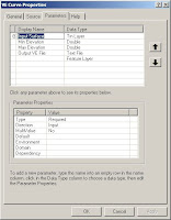
Figure 2: Add parameters to the script

Remember that the order the parameters show in this dialog is the order they are passed to your code. This means that the first parameter showing here will be accessed in your code through the sys.argv[1] system variable.

You will also need to make sure that you update all the Parameter Properties such as ensuring input and output data sets are assigned accordingly and that Dependencies are also assigned. This last one comes into play in situations such as the requirement to select from a list of fields.

Now when you double click on the script in the toolbox you should see a dialog something like that shown in Figure 3.

Figure 3: Tool dialog for our Script

Now you should have a workable tool that will produce a volume elevation curve from an existing containment TIN.  The intent of this post is not to show you how to do VE Curves but to give you a starting point for creating your own custom script based tools in ArcGIS.  Hope you find it useful.

ArcGIS and Volume Elevation Curves

I have been thinking about doing this blog for some time and have finally found the time to get to it. I have been doing volume/elevation curves for engineers for some time and have performed them in a few different applications but ArcGIS Desktop does one of the best jobs.

The premise of this particular curve scenario is one in which a tailings pond is being considered for a mining operation (any mining operation). The geotechnical engineers or geologists have a calculated number for the metric output for the mine over a 20 year period and need to make sure that a tailings pond will accommodate this number. Here is my take on the steps involved in performing a VE curve analysis using ArcGIS and 3D Analyst. Keep in mind I am not an engineer or a geologist and, even though I have performed this analysis hundreds of times, it was always double checked by one of these professionals.

Step 1: Creating the base surface.
Assuming you have a decent DEM for the area in question you will need to import it into ArcGIS as a TIN surface. This can be done using the one of the conversion utilities in Arc such as Raster to TIN under the 3D Analyst toolbar. Assuming the data is currently in an ASCII xyz file you will need to import it as a raster first then perform the Raster to TIN function. The resultant surface will be used for determining the containment area of the tailings pond and for performing the volume calculations at a series of elevations starting at the floor of the proposed tailings area and going to the top of the containment. This top elevation will be roughly determined by the desired containment volume and the practical height of the dam.

Step 2: Create the dam surface
The dam surface can be created in a number of different ways. For the purposes of this exercise we will create the dam in ArcGIS. To do this we will start with a center-line that is placed across the opening of the tailings area as discussed in Step 1. The line can be digitized into a "clean" shapefile or geodatabase feature set. You must ensure that this line crosses well over the desired elevation contour that represents the top elevation of the tailings containment. This will ensure that the resultant dam footprint overlaps the containment area. The resultant data set will need a field for elevation because the dam will be a 3D model used to finish the containment surface.

Figure 1a: Dam Geometry		Figure 1b: Dam TIN

Once the centerline has been established, an offset will be needed to create a practical crest for the dam. A typical offset might be 5 meters to create a 10 meter crest. Next the front and back slopes of the dam must be created. This can be accomplished by offsetting the crest to both the front and back by a predetermined distance (see Figure 1a). Because the faces of the dam are usually planar surfaces a single offset is usually adequate. The trick is figuring out how far to offset the lines. To do this you can look at the crest height and, using the slope of the dam face, determine how far to offset the line so that the outside limits fall below the lowest elevation in the containment surface. For example, if the dam height is 50 meters and the slope is proposed at 2:1 then an offset of 150 meters will ensure that the outside line is well below the containment surface (75 meters as in Figure 1) . This step will be needed both in front and behind the dam because the dam is used for both the tailings containment surface and to establish the footprint of the dam. Finally, convert these features to a new TIN surface using the 3D Analyst dropdown menu Create Tin from Features... It is a best practice to look at the new dam surface and the underlying elevation surface in ArcScene to ensure that the dam side slopes extend well below the Elevation surface (see Figure 2).

Figure 2: Dam Surface through Elevation Surface

Step 3: Containment Outline

The next step is fairly straight forward. You need to acquire the area outline of the tailings containment for given "ultimate dam" height. This requires that you create a planar surface at this elevation.

Figure 3a: Features for Planar Surface		Figure 3b: Tin Difference Polygons

You can do this by creating a new data set (shapefile or geodatabase feature set) and add it to the your map. Remember, you will need to assign a valid projection to this surface or you won't be able to create the necessary TIN surface. Now do the following:

1. Add a field to the data set for the elevation.
2. Establish the maximum extents for the containment by looking at the dam location and any contour or elevation information available
3. digitize a few perpendicular lines covering the entire area (similar to how you created the dam geometry - see Figure 3)
4. Assign an elevation to each of the lines. This will be the maximum elevation of the containment area which is usually the height of the dam minus an appropriate "free-board" or "draw-down".
5. Create a TIN surface from the this new data set.
6. Run the TIN Difference function from the 3D Analyst toolbox using the planar surface as Input TIN 1 and the elevation surface created in Step 1 as Input TIN 2.
   

The resultant data set will contain the outline of the tailings containment but will be "open" at where the dam should be (see Figure 3b).

Step 4: Create Dam Footprint
This is s very simple and short step. To create the dam footprint you simply use the TIN Difference tool and assign the dam TIN you created in Step 2 as Input TIN 1 and the underlying "DEM" TIN as Input TIN 2. This will give you a number of polygons showing the difference in volume between the two surfaces. The most important polygon will be the one showing the Greater Than area which will include the portion of the DAM above the underlying elevation surface. You may also need to dissolve some of the areas that show "No Change" values to make the polygon complete. Now simply edit this new "Difference" or "Dissolved Difference" data set and remove the polygons that do not include the dam "Toe".

Figure 4a: Dam/Surface Difference		Figure 4b: Dam Toe

Step 5: Close Containment Polygon
To close the containment polygon from Step 3, you can simply run a "Merge" on the new "Dam Toe" data set and the "Containment Difference" data set. You may need to expand the "Dam Toe" dataset to cross the appropriate containment polygon to ensure that the merge is successful and you have only one polygon for the containme nt in the end. Now edit this new data set and remove all the polygons that are not your tailings containment area.

Note: the step of stretching the dam toe is likely due to the detail and accuracy of the underlying DEM.

Step 6: Create the containment TIN for volume elevation analysis
Next you will need to create a surface that describes the containment area of the underlying elevation surface with the appropriate dam face in place. This can be done as follows:

1. Using the containment area polygon created in Step 4, create a raster with the Polygon to Raster tool where each cell has a value of 1
2. Using the Map Algebra or Times tools in Spatial Analyst, multiply this containment raster with the underlying elevation raster to create an elevation raster of only the containment area.
3. Convert this new elevation raster to points (Raster to Point)
4. Create the inside face of the dam
• Overlay dam outline from Step 4 and the Dam Geometry from Step 2
• Offset inside edge of dam crest a number of times so that several end up within the outline of the dam.
• Adjust the elevation of each line so that it lies at the appropriate slope within the face of the dam. (e.g. 2:1)
• Trim each line so that it does not extend past the outline of the dam
• Remove all lines that are not part of the inside face of the dam
5. Create a new TIN surface that includes the elevation points created here and the new inside dam face.
   

Figure 5a: Containment Features		Figure 5b: TIN from Features

Step 7: Create Volume Elevation Curve

You can now create a volume elevation curve. The best way to accomplish this is by using the Area and Volume analysis tool under the 3D Analyst tool bar as follows:

1. Open the Area and Volume tool from the 3D Analyst toolbar
2. Assign the new containment surface as Input surface
3. Set the Height of plain to be the same as Z min
4. Select Calculate statistics below plane
5. Z factor = 1
6. Select Save/append statistics to text file and select an appropriate location for the file
7. Click Calculate statistics
8. Increase Height of plane by a predetermined amount (e.g. 1o meters). This will likely be determined by the number of points required to create a good curve (typically 8 to 12 points is good)

Figure 6: Area and Volume Statistics Tool

You will now need to open the text file you created and modify the file so that it can be used in excel. The Area and Volume tool writes a number of statistics we don't need like 2D and 3D areas so you will need to remove these. At the same time you will need to create a comma delimited file that can be opened into columns in Excel. In the end you need only the Elevation and Volume items for each iteration in the previous steps. Save the file and open in Excel.

You will now need to add column headers and create the curve. To do this select the Insert -> Chart -> Scatter Chart. When prompted select your data for the chart. You will likely need to switch the columns in the appropriate series so that the volume runs along the X axis and the elevation along the Y. In the end you should have a decent looking VE curve.

Figure 7: Volume Elevation Curve
I hope this was helpful to those that may be new to this process. Please stand by and I will try to add other useful tutorials in the future.